PivotTable VII: – Conditional formatting gets even better, or visualizing your data in PivotTables
数据透视表VII －条件格式使数据透视表变得更好，数据更形象化

In a series of previous articles I introduced the new conditional formatting capabilities in Excel 12 (see here for the whole series of posts). Today I want to add one more article to the series, which is the work we have done to make conditional formatting work really well in Excel PivotTables. This is an area that I love to show people, because the work we have done reduces a formerly-tricky task down to a few clicks.
在我之前一系列的文章中，我介绍了Excel 12里面的条件格式。今天，我想在此系列里再增加一篇文章，那就是我们在Excel数据透视表里使用条件格式所作的努力。这是一个我乐意给人们展示的领域，因为我们所作的工作将以前难以完成的任务简化为非常简单的操作。

The first point I want to make is that all the features we added around new types of conditional formatting (data bars, colour scales, icon sets, etc.), new rules (top 10, below average, etc.), and new UI are available for use on PivotTables. However, we did not stop there. To provide a great experience with conditional formatting inside PivotTables, we now associate the conditional formatting rules to the structure of the PivotTable instead of to the cells. What this means is that as users work with PivotTables (adding and removing fields, refreshing the data, expanding and collapsing levels, Pivoting fields between rows and columns, grouping fields, etc.), the formatting tracks the cells in the PivotTable appropriately, so the users don’t need to worry about what is happening to the formatting – things just work, and they can focus on analyzing their data instead. Let’s walk through an example.
首先一点我需要说明的是，关于条件格式新格式（数据条，颜色比例，图标，等等），新规则（前10，均值之下，等等），以及新用户界面等方面增加的所有特点，在数据透视表里面都是可用的。然而，我们并没有就此满足。为了在数据透视表里面提供一个强大的条件格式体验，我们现在将条件格式的规则与数据透视表联系起来，而不是与单元格了。这意味着当用户操作数据透视表时（添加和删除字段，刷新数据，展开和折叠层次，在行与列之间透视字段，组合字段，等等），格式将恰当地追踪数据透视表里的单元格，因此用户不必担心格式会发生什么变化——照常运转，他们可以侧重于分析他们的数据。我们来看一个例子吧。

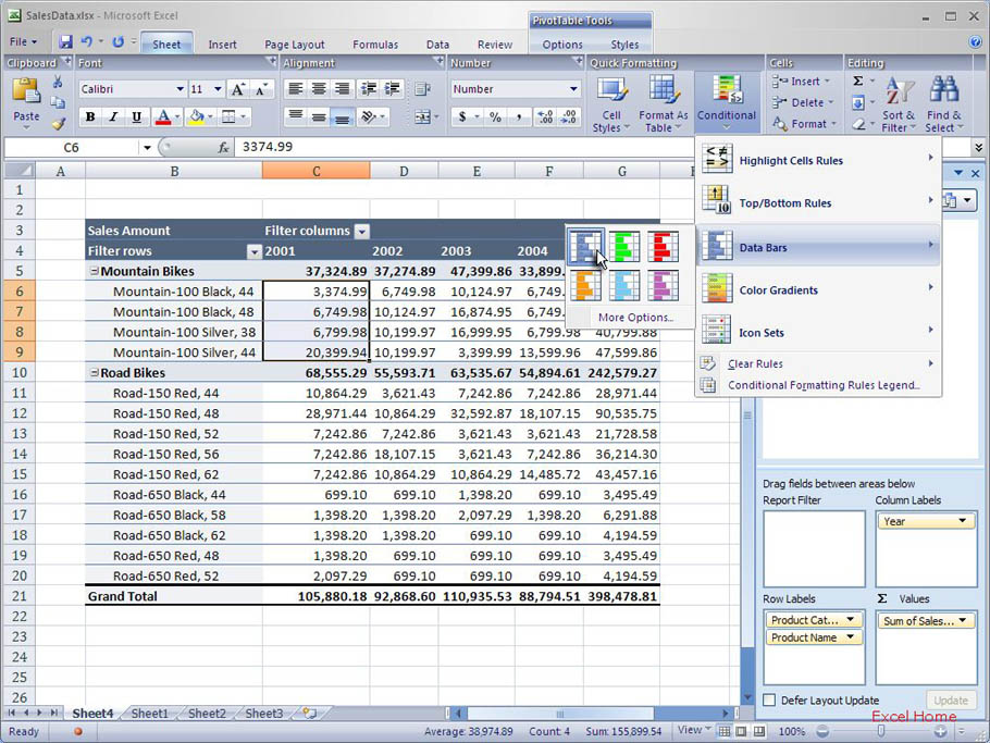
In the PivotTable below I’m looking at sales for different bike models, and I have arranged my report so that I have a column with sales data for each year. To make it easier to visually compare the sales of various bike models, I want to apply conditional formatting to the sales values. In the same way as I would when conditionally formatting “ordinary” (i.e. non-PivotTable cells), I select some cells containing sales values …
在下面的数据透视表里，我在看不同型号自行车的销售情况，我已经做好了我的报告，其中一列是每年的销售数据。我想要将条件格式应用到这些销售数据上，将不同型号自行车销售情况的比较变得形象化。就象设置“普通”（例如，非数据透视表单元格）的条件格式一样，我选择一些包含销售数据的单元格……

… and then I use the ribbon to add a Data Bar format which helps users quickly scan their data to compare values and find outliers.
……然后，我使用Ribbon来添加Data Bar格式，使用户快速浏览他们的数据时就可以比较数据并且找到突出者。

With two clicks, the conditional formatting is now applied to the cells I selected.
点击两次，条件格式就被应用到我所选单元格区域上了。

This is helpful, since I can now easily get a much better sense as to the relative sizes of the numbers I have selected, but oftentimes what I actually want is to apply the conditional formatting to *all* cells displaying bike sales. In this example, I might want to compare mountain bikes with road bikes using the same conditional formatting rule, but I want to avoid formatting subtotals (such as the total for the entire Mountain Bike category), since they would skew the results. You might be thinking “that’s going to take a lot of multiple-selection, especially on big PivotTables with a lot of levels.” To make it very easy to choose the “scope” of a conditional formatting rule in a PivotTable, Excel 12 provides some “on-object-UI” (OOUI) which gives you the choice of which scope you meant for the rule to be applied to (by scope I mean which set of cells get the conditional formatting).
这一招非常实用，因为我现在可以轻易地获得关于我所选择数字的相对大小概念。但是，我时常需要将该条件格式应用到显示自行车销售的所有单元格上。在本例中，我可能想用相同的条件格式规则来比较山地车和道路车，但是我想避开小计（例如整个山地车品类的总数），因为它们可能会弄乱结果。你可能会想“需要做很多个多区域选择，特别是有很多层次的大数据表”。为了使在数据透视表里选择条件格式“范围”变得非常简单，Excel 12提供一些“on-object-UI”（OOUI，译者，对象上的用户界面），让你选择你想要应用的范围（我想设置条件格式的单元格区域）。

上一篇：excel表格制作教程：Excel2007的自定义工作表函数（第一部分） 下一篇：表格制作快速入门：对编辑公式功能的改进Part 2

郑重声明：本文版权归原作者所有，转载文章仅为传播更多信息之目的，如作者信息标记有误，请第一时间联系我们修改或删除，多谢。