Today, I would like to cover some of the improvements we made in Excel 12 to make PivotTables easier to read and explore.
今天，我介绍一下Excel 12的一些改进，这些改进使得数据透视表更易于阅读与理解。

Expand Collapse
One of the nice exploration features of PivotTables is the ability to expand and collapse items in order to view values at different levels of detail. In Excel 12, we have added expand/collapse indicators to the PivotTable to make it easy to discover when there are more details to explore (and to make it obvious that this feature even exists!). The expand indicator is a “+” and the collapse indicator is a “-”.
展开折叠
数据透视表中一个值得探索的特征就是展开和折叠项目的功能，使用户能够按照不同的明细等级察看数据。在Excel 12 里，我们给数据透视表增加了展开/折叠指示器，让用户很容易就能看出是否含有隐藏的明细数据。这个展开指示器是一个“+”，折叠指示器是一个“-”。

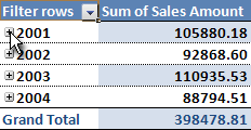
Let’s look at an example. In the PivotTable below, I have added three fields to the row area and the sales amount field to the values area. Currently only items of the first field, year, are showing. To display the details below 2001, all I have to do is to click the expand indicator:
让我们来看一个例子。在数据透视表的下面，我已经添加三个字段到行区域，销售额字段添加到值区域。通常只有第一个字段的项目“年份”显示出来。为了显示2001下面的明细数据，我们需要点击展开指示器。

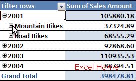
And now I’m looking at the sales amount for each product category in 2001:
现在，我们可以看到2001下面每一个产品种类的销售额：

To go to a lower level of detail, I can expand mountain bikes as well and I get the sales amount for each bike model:
为了看到下一级明细数据，我可以展开“山地自行车”，从而得到每款自行车的销售额：

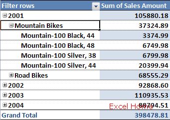
Note that I am now at the lowest level of my “hierarchy”, so there are no expand or collapse indicators. The indicators do not print by default, and they can be turned off altogether once you are done exploring the data and are getting ready to present the result.
我现在位于最底级的层级里，所以这里没有展开或折叠指示器。指示器在默认的情况下是不会被打印出来的，一旦你完成探究这些数据并做好显示结果的准备，那么这个指示器就会自动关掉。

Compact Axis
Many of you have probably noticed that the PivotTables in Excel 12 look more “compact” than a PivotTable in current Excel versions. Probably the easiest way to explain this is with a few pictures. Here is an Excel 12 PivotTable with three fields on the row axis.
Compact Axis
大家可能已经注意到Excel 12 的数据透视表看起来比当前的Excel版本的数据透视表更加紧凑。图片就是最好的证明。这是一个Excel 12 的数据透视表，在行轴上有三个字段。

And here is the same PivotTable in Excel 2003.
下面是同一个数据透视表在Excel 2003中的样子。

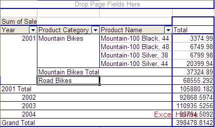
To significantly improve the readability of PivotTables, we have added a new layout option for displaying items in the row area, which the team refers to as “compact”. In the Excel 12 screenshot above, you’ll notice that items from all of the three different fields in the row area are displayed in a single column. To distinguish between items from different fields, Mountain Bikes is indented under 2001 and the individual mountain bike models are indented even further under Mountain Bikes. One of the key benefits of this feature is that PivotTable row labels take up far less room on your screen, so that there is much more room for your numbers.
为了有效的改进数据透视表的可读性，我们增加了一个新的布局选项，它可以显示行区域的项目，这组选项称为“compact”。在上面的Excel 12 截图中，你会注意到行区域中的三个不同的字段的项目显示在同一列上。为了区别不同字段的项目，山地自行车在2001下面缩进，而各种山地自行车款式也在山地自行车之下再缩进。这个特征的主要好处就是在你的屏幕中数据透视表的行标签占据更少的空间，所以有更多的空间让你放置你的数据。

上一篇：excel怎么做表格：专业图表轻松做(续)+Excel2007键盘访问模 下一篇：excel vba教程：Excel自定义数字格式的经典应用

郑重声明：本文版权归原作者所有，转载文章仅为传播更多信息之目的，如作者信息标记有误，请第一时间联系我们修改或删除，多谢。