PivotTables part 2: Creating summary reports made easy
数据透视表2：轻松创建综合报告

One of the goals we had for our PivotTable work in Excel 12 was to make creating PivotTables a much more approachable task. In this post, I would like to walk through an example of creating a PivotTable in order to highlight the changes we have made in Excel 12. In general, we tried to make the process simpler and more intuitive.
让用户很方便、很直观的创建数据透视表是我们的一个目标，我们已经在Excel 12 中实现了这个目标。在这篇文章，为了重点说明我们在Excel 12 中对数据透视表作出的改变，我创建一个数据透视表作为例子。通常，我们试图使得操作过程简单而且直观。

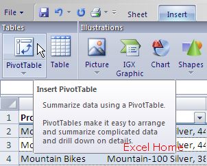
As I said in the previous post, PivotTables are great for summarizing large amounts of data. For example, a user might have a table full of sales data (contained in a query table, that they copied from elsewhere, that they have been typing into the grid over time, etc.) that contains products, sales figures, product categories, etc., and might want to see a summary of sales grouped by product and product category. This is exactly the sort of thing that is easy to create with a PivotTable. To start, the user needs to tell Excel they want to create a PivotTable. There are two places they can do this. First, on the Insert tab, where the first button in the ribbon is an inset PivotTable button.
正如我在以前的文章中所说，数据透视表主要用于处理大量的数据。例如，某个用户可能有一个填满销售数据的列表，包含产品、销售指数、产品种类等等，并且该用户想通过产品及产品种类看到各个销售组的销售概要。通过创建数据透视表这是件很容易实现的事情。回到出发点，用户需要告诉Excel，他们想要创建数据透视表。创建数据透视表有两种方式：第一、在“插入”标签上，在 ribbon 里的第一个按钮就是“插入数据透视表”按钮。

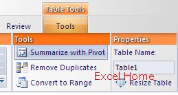
Second, on the Table tab (the tab that shows up when I am working with a table of data), we have added a command to “Summarize With Pivot”. This is essentially the same command, except when you use this command, we know that you want the table you are working with to be the data source for the PivotTable.
第二、在“列表”标签上（当我激活数据表时这个标签才会显示出来），我们已经附加一个命令到“Summarize With Pivot”。从本质上讲，这是相同的命令，除非当你使用这个命令时，我们知道你想把你正在操作的列表作为数据透视表的源数据。

Once the user selects one of these commands, they are presented with a new dialog for creating PivotTables. This dialog replaces the existing multistep wizard with a simple dialog that only presents the user with the most necessary choices … our usability research showed that a lot of users never made it past the wizard due to the complexity of choices required. (Note, there are probably some out there wondering about whether they can still pivot against multiple consolidation ranges, etc. … the answer is yes. The existing wizard is still available for advanced users that want to take advantage of its functionality; it just isn’t the mainline UI):
一旦用户选择这两个命令的其中之一时，会出现一个创建数据透视表的新对话框。这个简单的对话框取代了现有的多级向导，只显示用户必需的选项……我们的可用性调查报告表明：由于繁琐的选择条件，许多用户从来不按照向导的步骤创建数据透视表。（注：可能会有人怀疑这样的数据透视表是否仍然可以随着多重合并区域的变动而变。回答是肯定的。现有的向导仍然适用于想利用这个功能的高级用户，但它已经不处在主界面上了。）

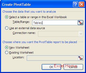
In our example, because we had a table selected when we created the PivotTable, all our user has to do is to click OK and the PivotTable is created – that’s a total of two clicks. If the user wanted to work with data external to Excel, they would simply select “Use an external data source” and select the external data connection they would like to use from the drop down. (Note that in the Table/Range refedit control, you can now type “structured references” to tables or parts of tables in addition to cell references. This is true for most of the refedit controls in Excel, and is another small but powerul addition to the product. See this post for more on structured referencing.)
在我们的例子里，因为当我们创建数据透视表时已经选择了一个列表，所以用户所要做的就是点击“OK”，那么数据透视表就创建完成了——这总共只需要点击两次鼠标。如果用户想要引用外部数据到Excel，只需要简单的选择“使用外部数据源”并从下拉列表中选择他们想要用的外部数据连接。（注：在列表/范围refedit controns，除了单元格引用之外，你还可以键入“structured references（成形的引用）”。在 Excel中，多数的refedit controns都是可以实现的，这也是另一个小而高效的附加功能。这篇文章（ this post）可以看到更多的关于成形引用的介绍。）

上一篇：表格制作excel教程：SmartArt 图形和样式（二） 下一篇：excel表格制作教程：Excel 2007新知

郑重声明：本文版权归原作者所有，转载文章仅为传播更多信息之目的，如作者信息标记有误，请第一时间联系我们修改或删除，多谢。